cor(mtcars$mpg, mtcars$hp)[1] -0.7761684This tutorial focuses on simple linear regression. This tutorial will focus on different methods in conducting a simple linear regression in R. You only need to do section 1 and 2 to learn how to do SLR in R.
For this tutorial, we will use the mtcars data set and comparing the the mpg (dependent) variable with the hp (independent) variable.
Through out this tutorial, we use certain notations for different components in R. To begin, when something is in a gray block, _, this indicates that R code is being used. When I am talking about an R Object, it will be displayed as a word. For example, we will be using the R object mtcars. When I am talking about an R function, it will be displayed as a word followed by an open and close parentheses. For example, we will use the mean function denoted as mean() (read this as “mean function”). When I am talking about an R argument for a function, it will be displayed as a word following by an equal sign. For example, we will use the data argument denoted as data= (read this as “data argument”). When I am referencing an R package, I will use :: (two colons) after the name. For example, in this tutorial, I will use the ggplot2:: (read this as “ggplot2 package”) Lastly, if I am displaying R code for your reference or to run, it will be displayed on its own line. There are many components in R, and my hope is that this will help you understand what components am I talking about.
Linear Relationship
SLR via lm()
Multivariable Linear Regression
MLR via lm()
Questions
When we are comparing two continuous variables, we are measuring the association between them. We want to know how does one variable change when the other variable increases or decreases. There are two methods to measure this association: a correlation or linear regression.
The correlation coefficient is a statistic used to measure the association between 2 variables. The value range from -1 to 1. To compute the correlation coefficient, use the cor(). You will only need to specify the x= and y= which indicate the vectors of data to compute the correlation:
cor(mtcars$mpg, mtcars$hp)[1] -0.7761684With linear regression, we are trying to fit a line such that all the points are closest to the line as possible. Below is the scatter plot of hp vs mpg
ggplot(mtcars, aes(hp, mpg)) + geom_point() + theme_bw()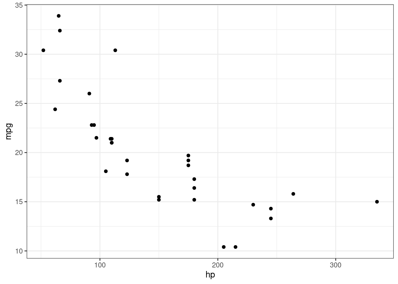
As you can see, there is a negative association. As hp goes up, mpg goes down. What we want to do is fit a line where all the points are closest to the line. The next four plots demonstrates how a line is fitted. Linear regression searches for a line until the distance between all the points and the line are smallest possible. The fourth plot with the blue line indicates the best fit line.
ggplot(mtcars, aes(hp, mpg)) + geom_point() + theme_bw() +
geom_function(fun=yy, args = list(m = -.205, b = 50)) 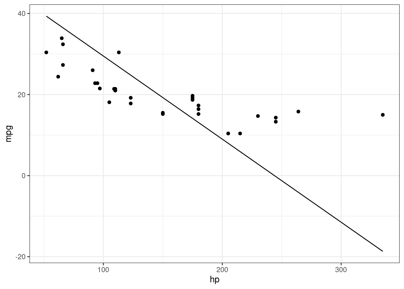
Notice how the points at the end of the plot are further away from the line.
ggplot(mtcars, aes(hp, mpg)) + geom_point() + theme_bw() +
  geom_function(fun=yy, args = list(m = -.013, b = 20))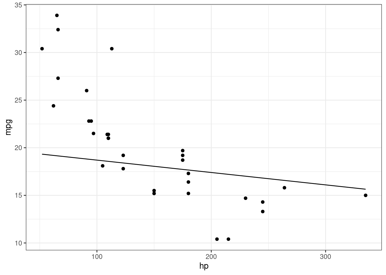
This is much better, but the points at the beginning are further away.
ggplot(mtcars, aes(hp, mpg)) + geom_point() + theme_bw() +
geom_function(fun=yy, args = list(m = -.10, b = 35)) 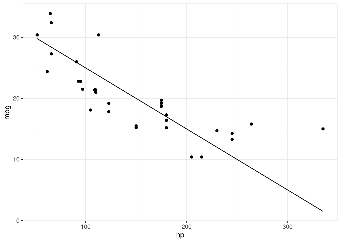
This plot provides a better fit of the data.
ggplot(mtcars, aes(hp, mpg)) + geom_point() + theme_bw() +
  geom_smooth(method = "lm", se = F)
`geom_smooth()` using formula = 'y ~ x'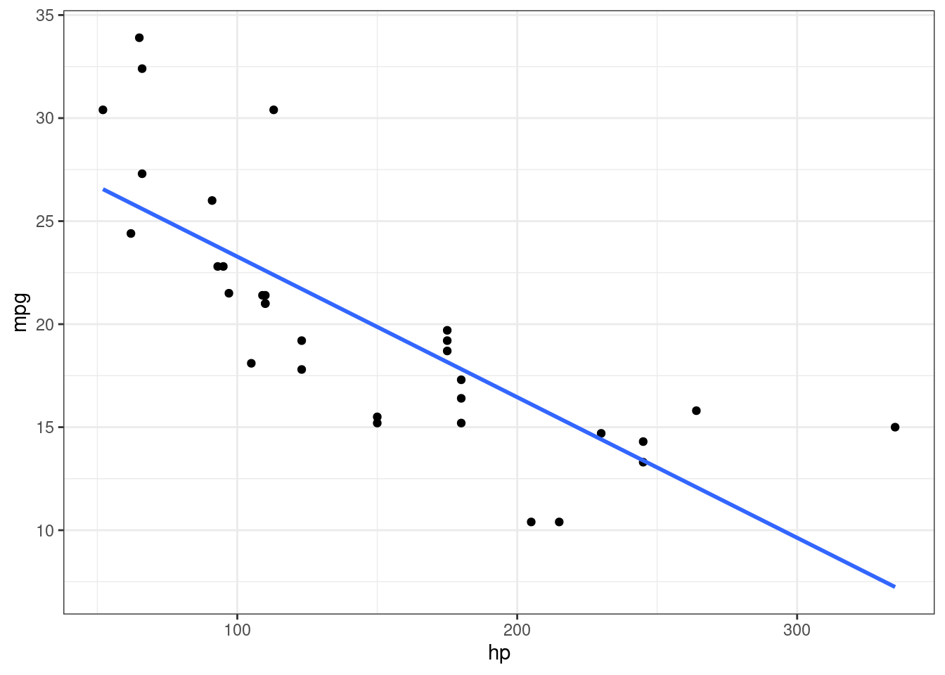
This contains the fitted line from the linear regression.
Mathematically, we are try trying to find the values for an equation of a line that fits the data. The equation of the line for the \(i^{th}\) point is
\(Y_i= \beta_0 + \beta_1 X_i + \varepsilon_i,\)
where \(Y_i\) is the \(i^{th}\) outcome, \(X_i\) is the \(i^{th}\) predictor, \(\epsilon_i\) is the \(i^{th}\) error term, \(\beta_0\) is the intercept, and \(\beta_1\) is the slope. The error term is the distance between the line and the point. Therefore, we want to minimize the error term:
\(\varepsilon_i = Y_i-\beta_0 -\beta_1 X_i\)
Because some of the error terms are negative (points are below the line), we will need to square it. Lastly, we want to minimize all the points, so we add all observations together and minimize the following least-squares formula:
\(\sum_{i=1}^n(Y_i-\beta_0 -\beta_1 X_i)^2\)
We will need to find the values of \(\beta_0\) and \(\beta_1\) that minimizes the least-squares formula. We can use the Ordinary least-squares (OLS) or the Maximum Likelihood Estimation (MLE) estimators to obtain the these estimates.
lm()Fitting the model means finding the estimates of \(\beta_0\) and \(\beta_1\) that minimizes the least-squares formula, which is denoted with hat: \(\hat \beta_0\) and \(\hat \beta_1\). In R, we can obtain these estimates using the lm(). The lm() function only needs the formula= and the data= as inputs. The output of the lm() is an lm R class that contains information about the model.
To conduct a linear regression where mpg is the dependent variable and hp is the independent variable. Then, we will store the output from the lm() in the R object xlm.
xlm <- lm(mpg~hp, data = mtcars)To view the summary table of coefficients from the lm(), you will need to use the summary():
summary(xlm)
Call:
lm(formula = mpg ~ hp, data = mtcars)

Residuals:
    Min      1Q  Median      3Q     Max
-5.7121 -2.1122 -0.8854  1.5819  8.2360

Coefficients:
            Estimate Std. Error t value Pr(>|t|)
(Intercept) 30.09886    1.63392  18.421  < 2e-16 ***
hp          -0.06823    0.01012  -6.742 1.79e-07 ***
---
Signif. codes:  0 '***' 0.001 '**' 0.01 '*' 0.05 '.' 0.1 ' ' 1

Residual standard error: 3.863 on 30 degrees of freedom
Multiple R-squared:  0.6024,    Adjusted R-squared:  0.5892
F-statistic: 45.46 on 1 and 30 DF, p-value: 1.788e-07summary(xlm)
Call:
lm(formula = mpg ~ hp, data = mtcars)

Residuals:
    Min      1Q  Median      3Q     Max
-5.7121 -2.1122 -0.8854  1.5819  8.2360

Coefficients:
            Estimate Std. Error t value Pr(>|t|)
(Intercept) 30.09886    1.63392  18.421  < 2e-16 ***
hp          -0.06823    0.01012  -6.742 1.79e-07 ***
---
Signif. codes:  0 '***' 0.001 '**' 0.01 '*' 0.05 '.' 0.1 ' ' 1

Residual standard error: 3.863 on 30 degrees of freedom
Multiple R-squared:  0.6024,    Adjusted R-squared:  0.5892
F-statistic: 45.46 on 1 and 30 DF,  p-value: 1.788e-07
The results from the summary() provide statistics on the residuals, a coefficient table with corresponding hypothesis test, and other relevant statistics for model fit.
Focusing on the coefficient table, it provides information for each variable (labeled in the rows section). For each regression coefficient, the table provides an “Estimate”, “Std. Error”, “t value”, and “Pr(>|t|)”. The p-value corresponds to the following hypothesis test:
\(H_0: \beta = 0\),
and
\(H_1: \beta \neq 0\).
Simple linear regression uses a model with one independent variable:
\[ Y = \beta_0 + \beta_1 X_1. \]
The multivariable linear regression extends the model to include more than independent variable:
\[ Y = \beta_0 + \beta_1 X_1 + \beta_2 X_2 + \cdots + \beta_p X_p, \]
and in matrix form:
\[ Y = \boldsymbol X ^ \mathrm T \boldsymbol \beta, \]
where
\[ \boldsymbol \beta = \left( \begin{array}{c} \beta_0 \\ \beta_1 \\ \beta_2 \\ \vdots \\ \beta_p \end{array} \right) \]
and
\[ \boldsymbol X = \left(\begin{array}{cc} 1 & X_{11} & X_{21} & \cdots & X_{p1}\\ 1 & X_{12} & X_{23} & \cdots & X_{p2}\\ \vdots & \vdots & \vdots & \ddots & \vdots \\ 1 & X_{1n} & X_{2n} & \cdots & X_{pn}\\ \end{array} \right). \]
To fit the data to the model, we search for values of \(\hat \beta\) that minimizes the least-squares formula:
\[ \sum^n_{i=1} \left( Y_i - \boldsymbol X_i ^ \mathrm T \boldsymbol \beta \right)^2 \]
For the rest of the tutorial, we will go over how to find the estimates of \(\beta\)
lm()First, we are interested in fitting the model below:
\[ mpg = \beta_0 + \beta_1 \cdot hp +\beta_2 \cdot cyl + \beta_3 \cdot wt + \beta_4 \cdot disp. \]
The outcome variable is mpg, and the independent variables are hp, cyl, wt, and disp. Fitting a multivariable linear regression in R is done with the lm(). We just need to specify the formula= and the data=. Similar to the simple linear regression model, the formula= contains the outcome on side of the ~ and the independent variables are on the other side. The independent variable are added to each other using the + operator. For example, the formula= is coded as
mpg ~ hp + cyl + wt + dispUsing the formula above, fit a model with the outcome variable is mpg and the independent variables are hp, cyl, wt, and disp from the mtcars data set.
xlm <- lm(mpg ~ hp + cyl + wt + disp, data = mtcars)Lastly, we can obtain organized output using the summary(). Obtain the summary for xlm.
summary(xlm)
Call:
lm(formula = mpg ~ hp + cyl + wt + disp, data = mtcars)

Residuals:
    Min      1Q  Median      3Q     Max
-4.0562 -1.4636 -0.4281  1.2854  5.8269

Coefficients:
            Estimate Std. Error t value Pr(>|t|)
(Intercept) 40.82854    2.75747  14.807 1.76e-14 ***
hp          -0.02054    0.01215  -1.691 0.102379
cyl         -1.29332    0.65588  -1.972 0.058947 .
wt          -3.85390    1.01547  -3.795 0.000759 ***
disp         0.01160    0.01173   0.989 0.331386
---
Signif. codes:  0 '***' 0.001 '**' 0.01 '*' 0.05 '.' 0.1 ' ' 1

Residual standard error: 2.513 on 27 degrees of freedom
Multiple R-squared:  0.8486,    Adjusted R-squared:  0.8262
F-statistic: 37.84 on 4 and 27 DF, p-value: 1.061e-10The estimated covariance matrix of \(\hat \beta\) can be obtained with the vcov() on an R object containing the output from the lm(). To obtain the covariance matrix of \(\hat \beta\) from xlm, use the vcov()
vcov(xlm) (Intercept) hp cyl wt disp
(Intercept) 7.603629375 2.005298e-03 -1.238326838 -1.777628876 2.462149e-02
hp 0.002005298 1.475440e-04 -0.003531738 0.001567700 -2.964271e-05
cyl -1.238326838 -3.531738e-03 0.430174318 0.017632767 -4.169713e-03
wt -1.777628876 1.567700e-03 0.017632767 1.031186716 -8.144097e-03
disp 0.024621488 -2.964271e-05 -0.004169713 -0.008144097 1.375181e-04Focusing on the coefficient table from the summary(), it provides information for each variable (labeled in the rows section). For each regression coefficient, the table provides an “Estimate”, “Std. Error”, “t value”, and “Pr(>|t|)”. The p-value corresponds to the following hypothesis test:
\(H_0: \beta_j = 0\),
and
\(H_1: \beta_j \neq 0\).
The faithful data set in R contains information on eruptions time and waiting time. Describe the relationship between waiting (independent) and eruptions (dependent).
The cats data set from the MASS package contains information of cat body weight (kg; Bwt) and heart weight (g; Hwt). Fit a model to see if there is a significant association between body weight (predictor) and heart weight (outcome).
Due May 14 @ 11:59 PM