Joint Distribution Functions
Learning Outcomes
Marginal Distributions
Conditional Distributions
Independence
Expectations
Covariance
Joint Distributions
Joint Distribution Functions
- A joint distribution of two random variables \(X\) and \(Y\) describes how they behave together.
- It tells us the probability (discrete case) or probability density (continuous case) assigned to different pairs \((x,y)\).
- Think of it as a “probability landscape” in 2D:
- On a grid for discrete outcomes.
- As a surface over the plane for continuous outcomes.
- On a grid for discrete outcomes.
Discrete Joint Mass Function
Definition: If \(X\) and \(Y\) take values in countable sets \(\mathcal{X}, \mathcal{Y}\), then
\[ p_{X,Y}(x,y) = \Pr(X=x, Y=y), \quad (x,y)\in \mathcal{X}\times \mathcal{Y}. \]
Properties:
- Non-negativity: \(p_{X,Y}(x,y) \ge 0\) for all \((x,y)\).
- Normalization:
\[ \sum_{x\in \mathcal{X}} \sum_{y\in \mathcal{Y}} p_{X,Y}(x,y) = 1. \]
Continuous Joint Density Function
Definition: If \((X,Y)\) is continuous, it is described by a joint density \(f_{X,Y}(x,y)\) such that for any region \(A \subseteq \mathbb{R}^2\):
\[ \Pr((X,Y)\in A) = \iint_A f_{X,Y}(x,y)\, dx\,dy. \]
Properties:
- Non-negativity: \(f_{X,Y}(x,y) \ge 0\) everywhere.
- Normalization:
\[ \int_{-\infty}^\infty\int_{-\infty}^\infty f_{X,Y}(x,y)\,dx\,dy = 1. \]
More than 2 RV’s
Let \(X_1, X_2, \dots, X_n\) be random variables.
Discrete case:
The joint pmf is
\[ p_{X_1,\dots,X_n}(x_1,\dots,x_n) = \Pr(X_1=x_1, \dots, X_n=x_n) \]Continuous case:
The joint pdf is
\[ f_{X_1,\dots,X_n}(x_1,\dots,x_n) \]
Simulate Bivariate Normal
Bivariate Normal Distribution
Code
library(MASS)
library(ggplot2)

# Parameters
mu <- c(0, 0)        # mean vector
sigma_x <- 2
sigma_y <- 1
rho <- 0.7           # correlation
Sigma <- matrix(c(sigma_x^2, rho*sigma_x*sigma_y,
                  rho*sigma_x*sigma_y, sigma_y^2), ncol = 2)

# Simulate data
set.seed(123)
n <- 2000
XY <- as.data.frame(mvrnorm(n = n, mu = mu, Sigma = Sigma))
names(XY) <- c("X", "Y")

# Scatter plot with density contours
ggplot(XY, aes(x = X, y = Y)) +
  geom_point(alpha = 0.3, color = "steelblue") +
  stat_density_2d(aes(z = ..level..), bins = 8,
                  geom = "polygon", alpha = 0.2, fill = "tomato") +
  theme_bw(base_size = 14)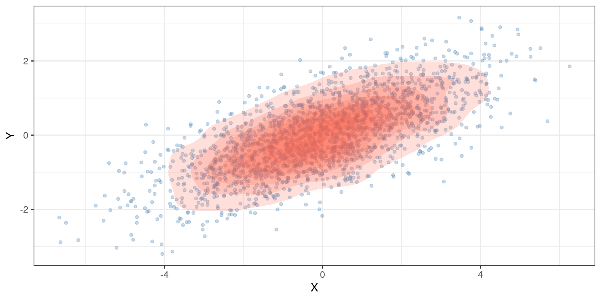
Marginal Density Function
Marginal Density Functions
A Marginal Density Function is density function of one random variable from a random vector.
Marginal Discrete Probability Mass Function
Let \(X_1\) and \(X_2\) be 2 discrete random variables, with a joint distribution function of
\[ p_{X_1,X_2}(x_1, x_2) = P(X_1=x_1, X_2 = x_2). \]
The marginal distribution of \(X_1\) is defined as
\[ p_{X_1}(x_1) = \sum_{x_2}p_{X_1,X_2}(x_1,x_2) \]
Marginal Continuous Density Function
Let \(X_1\) and \(X_2\) be 2 continuous random variables, with a joint density function of \(f_{X_1,X_2}(x_1,x_2)\). The marginal distribution of \(X_1\) is defined as
\[ f_{X_1}(x_1) = \int_{x_2}f_{X_1,X_2}(x_1,x_2)dx_2 \]
Example
\[ f_{X,Y}(x,y) \left\{\begin{array}{cc} 2x & 0\le y \le 1;\ 0 \le x\le 1\\ 0 & \mathrm{otherwise} \end{array}\right. \]
Find \(f_X(x)\)
Conditional Distributions
Conditional Distributions
A conditional distribution provides the probability of a random variable, given that it was conditioned on the value of a second random variable.
Discrete Conditional Distributions
Let \(X_1\) and \(X_2\) be 2 discrete random variables, with a joint distribution function of
\[ p_{X_1,X_2}(x_1, x_2) = P(X_1=x_1, X_2 = x_2). \]
The conditional distribution of \(X_1|X_2=x_2\) is defined as
\[ p_{X_1|X_2}(x_1) = \frac{p_{X_1,X_2}(x_1,x_2)}{p_{X_2}(x_2)} \]
Continuous Conditional Distributions
Let \(X_1\) and \(X_2\) be 2 continuous random variables, with a joint density function of \(f_{X_1,X_2}(x_1,x_2)\). The conditional distribution of \(X_1|X_2=_2\) is defined as
\[ f_{X_1|X_2}(x_1) = \frac{f_{X_1,X_2}(x_1,x_2)}{f_{X_2}(x_2)} \]
Example
Let the joint density function of \(X_1\) and \(X_2\) be defined as
\[ f_{X_1,X_2}(x_1,x_2)=\left\{\begin{array}{cc} 30x_1x_2² & x_1 -1 \le x_2 \le 1-x_1; 0\le x_1\le 1\\ 0 & \mathrm{elsewhere} \end{array}\right. \]
Find the conditional density function of \(X_2|X_1=x_1\).
Independence
Independent Random Variables
Random variables are considered independent of each other if the probability of one variable does not affect the probability of another variable.
Discrete Independent Random Variables
Let \(X_1\) and \(X_2\) be 2 discrete random variables, with a joint density function of \(p_{X_1,X_2}(x_1,x_2)\). \(X_1\) is independent of \(X_2\) if and only if
\[ p_{X_1,X_2}(x_1,x_2) = p_{X_1}(x_1)p_{X_2}(x_2) \]
Continuous Independent Random Variables
Let \(X_1\) and \(X_2\) be 2 continuous random variables, with a joint density function of \(f_{X_1,X_2}(x_1,x_2)\). \(X_1\) is independent of \(X_2\) if and only if
\[ f_{X_1,X_2}(x_1,x_2) = f_{X_1}(x_1)f_{X_2}(x_2) \]
Matrix Algebra
\[ A = \left(\begin{array}{cc} a_1 & 0\\ 0 & a_2 \end{array}\right) \]
\[ \det(A) = a_1a_2 \]
\[ A^{-1}=\left(\begin{array}{cc} 1/a_1 & 0 \\ 0 & 1/a_2 \end{array}\right) \]
Example
\[ \left(\begin{array}{c} X\\ Y \end{array}\right)\sim N \left\{ \left(\begin{array}{c} \mu_x\\ \mu_y \end{array}\right),\left(\begin{array}{cc} \sigma_x^2 & 0\\ 0 & \sigma_y^2 \end{array}\right) \right\} \]
Show that \(X\perp Y\).
\[ f_{X,Y}(x,y)=\det(2\pi\Sigma)^{-1/2}\exp\left\{-\frac{1}{2}(\boldsymbol{w}-\boldsymbol\mu)^T\Sigma^{-1}(\boldsymbol w-\boldsymbol\mu)\right\} \]
where \(\Sigma=\left(\begin{array}{cc}\sigma_y^2 & 0\\0 & \sigma_y^2\end{array}\right)\), \(\boldsymbol \mu = \left(\begin{array}{cc}\mu_x\\ \mu_y \end{array}\right)\), and \(\boldsymbol w = \left(\begin{array}{cc} x\\ y \end{array}\right)\)
Expectations
Expectations
Let \(X_1, X_2, \ldots,X_n\) be a set of random variables, the expectation of a function \(g(X_1,\ldots, X_n)\) is defined as
\[ E\{g(X_1,\ldots, X_n)\} = \sum_{x_1\in X_1}\cdots\sum_{x_n\in X_n}g(X_1,\ldots, X_n)p(x_1,\ldots,x_n) \]
or
\[ E\{g(\boldsymbol X)\} = \int_{x_1\in X_1}\cdots\int_{x_n\in X_n}g(\boldsymbol X)f(\boldsymbol X)dx_n \cdots dx_1 \]
- \(\boldsymbol X = (X_1,\cdots, X_n)\)
Expected Value and Variance of Linear Functions
Let \(X_1,\ldots,X_n\) and \(Y_1,\ldots,Y_m\) be random variables with \(E(X_i)=\mu_i\) and \(E(Y_j)=\tau_j\). Furthermore, let \(U = \sum^n_{i=1}a_iX_i\) and \(V=\sum^m_{j=1}b_jY_j\) where \(\{a_i\}^n_{i=1}\) and \(\{b_j\}_{j=1}^m\) are constants. We have the following properties:
\(E(U)=\sum_{i=1}^na_i\mu_i\)
\(Var(U)=\sum^n_{i=1}a_i^2Var(X_i)+2\underset{i<j}{\sum\sum}a_ia_jCov(X_i,X_j)\)
\(Cov(U,V)=\sum^n_{i=1}\sum^m_{j=1}Cov(X_i,Y_j)\)
Conditional Expectations
Let \(X_1\) and \(X_2\) be two random variables, the conditional expectation of \(g(X_1)\), given \(X_2=x_2\), is defined as
\[ E\{g(X_1)|X_2=x_2\}=\sum_{x_1}g(x_1)p(x_1|x_2) \]
or
\[ E\{g(X_1)|X_2=x_2\}=\int_{x_1}g(x_1)f(x_1|x_2)dx_1. \]
Conditional Expectations
Furthermore,
\[ E(X_1)=E_{X_2}\{E_{X_1|X_2}(X_1|X_2)\} \]
and
\[ Var(X_1) = E_{X_2}\{Var_{X_1|X_2}(X_1|X_2)\} + Var_{X_2}\{E_{X_1|X_2}(X_1|X_2)\} \]
Covariance
Covariance
Let \(X_1\) and \(X_2\) be 2 random variables with mean \(\mu_1\) and \(\mu_2\), respectively. The covariance of \(X_1\) and \(X_2\) is defined as
\[ \begin{eqnarray*} Cov(X_1,X_2) & = & E\{(X_1-\mu_1)(X_2-\mu_2)\}\\ & =& E(X_1X_2)-\mu_1\mu_2 \end{eqnarray*} \]
If \(X_1\) and \(X_2\) are independent random variables, then
\[ Cov(X_1,X_2)=0 \]
Correlation
The correlation of \(X_1\) and \(X_2\) is defined as
\[ \rho = Cor(X_1,X_2) = \frac{Cov(X_1,X_2)}{\sqrt{Var(X_1)Var(X_2)}} \]