Hypothesis Testing

Linear and Generalized Linear Models

Statistical Inference

1. Statistical Inference
2. Hypothesis Testing
3. Decision Making
4. Model Inference
5. Confidence Intervals
6. Power Analysis
7. Model Conditions

What is Statistical Inference?

• Drawing conclusions about a population based on a sample
• Population = entire group
• Sample = subset

Introduce the big idea: We want to make st

Two Main Types of Inference

1. Estimation
2. Hypothesis Testing

We’ll be focusing on two fundamental techniques in inference. First, estimating population values (like the mean), and second, testing claims about the population.

Estimation

• Point Estimate: Single best guess (e.g., \(\hat \beta_1\))
• Interval Estimate: Range likely to contain the true value

Point estimates are easy but not very informative. Intervals give us a sense of uncertainty, which is critical in inference.

Hypothesis Testing

• \(H_0\): No effect or difference
  
• \(H_1\): Some effect or difference
  
• We use sample data to support or reject \(H_0\)

Mention that \(H_0\) is the default assumption. We only reject it if the data give us strong enough evidence.

Key Concepts and Tools

• Sampling Distribution
• Central Limit Theorem
• Standard Error

These three concepts are foundational. Understanding them helps us assess how reliable our estimates are.

p-values

• Probability of observing data as extreme as this if \(H_0\) is true

• Misinterpretation of p-values is common.

• Emphasize: low p-value means data is unusual under \(H_0\).

Confidence Intervals

• A range where we expect the true value to fall

Clarify interpretation: it’s not about the probability the parameter is inside the interval, but about the method producing accurate intervals in the long run.

Hypothesis Testing

1. Statistical Inference
2. Hypothesis Testing
3. Decision Making
4. Model Inference
5. Confidence Intervals
6. Power Analysis
7. Model Conditions

Hypothesis Tests

Hypothesis tests are used to test whether claims are valid or not. This is conducted by collecting data, setting the Null and Alternative Hypothesis.

Null Hypothesis \(H_0\)

The null hypothesis is the claim that is initially believed to be true. For the most part, it is always equal to the hypothesized value.

Alternative Hypothesis \(H_1\)

The alternative hypothesis contradicts the null hypothesis.

Example of Null and Alternative Hypothesis

We want to see if \(\beta\) is different from \(\beta^*\)

Null Hypothesis	Alternative Hypothesis
\(H_0: \beta=\beta^*\)	\(H_1: \beta\ne\beta^*\)
\(H_0: \beta\le\beta^*\)	\(H_1: \beta>\beta^*\)
\(H_0: \beta\ge\beta^*\)	\(H_1: \beta<\beta^*\)

One-Side vs Two-Side Hypothesis Tests

Notice how there are 3 types of null and alternative hypothesis, The first type of hypothesis (\(H_1:\beta\ne\beta^*\)) is considered a 2-sided hypothesis because the rejection region is located in 2 regions. The remaining two hypotheses are considered 1-sided because the rejection region is located on one side of the distribution.

Null Hypothesis	Alternative Hypothesis	Side
\(H_0: \beta=\beta^*\)	\(H_1: \beta\ne\beta^*\)	2-Sided
\(H_0: \beta\le\beta^*\)	\(H_1: \beta>\beta^*\)	1-Sided
\(H_0: \beta\ge\beta^*\)	\(H_1: \beta<\beta^*\)	1-Sided

Hypothesis Testing Steps

1. State \(H_0\) and \(H_1\)
2. Choose \(\alpha\)
3. Compute confidence interval/p-value
4. Make a decision

Walk through the steps slowly with an example in mind. Emphasize that \(\alpha\) is a threshold, not the actual probability of error.

Rejection Region

• The rejection region is the set of all test statistic values that lead to rejecting \(H_0\).

• It’s defined by a significance level (\(\alpha\)) — the probability of rejecting \(H_0\), when it’s actually true.

Rejection Region

Decision Making

1. Statistical Inference
2. Hypothesis Testing
3. Decision Making
4. Model Inference
5. Confidence Intervals
6. Power Analysis
7. Model Conditions

Decision Making

Hypothesis Testing will force you to make a decision: Reject \(H_0\) OR Fail to Reject \(H_0\)

Reject \(H_0\): The effect seen is not due to random chance, there is a process contributing to the effect.

Fail to Reject \(H_0\): The effect seen is due to random chance. Random sampling is the reason why an effect is displayed, not an underlying process.

Decision Making: Test Statistic

\(\phi\) known

\[ ts = \frac{\hat\beta_j - \beta_j}{\mathrm{se}(\hat\beta_j)} \sim N(0,1) \]

\(\phi\) unknown

\[ ts = \frac{\hat\beta_j-\beta_j}{\mathrm{se}(\hat\beta_j)} \sim t_{n-p} \]

Decision Making: P-Value

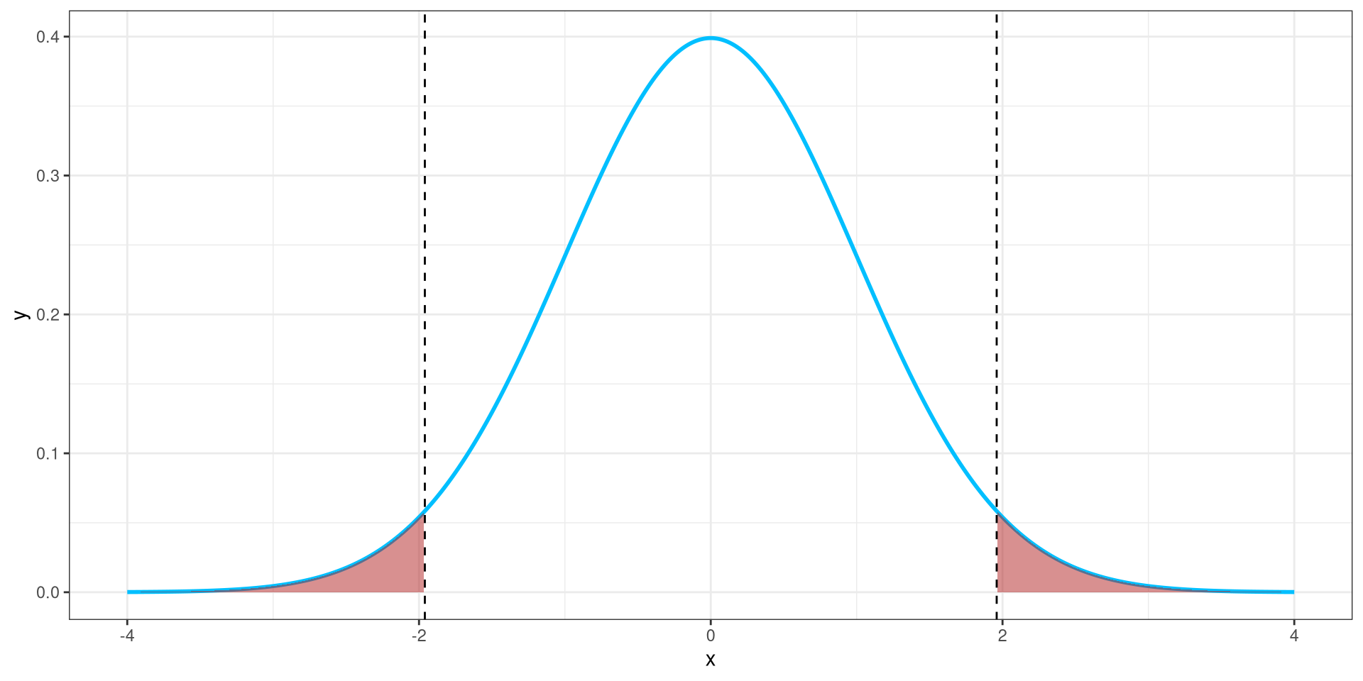
Two-Sided Test

\[ P(T > |ts|) = \int^\infty_{ts} f(t) dt + \int_{-\infty}^{ts} f(t) dt \]

One-Sided Test \[ P(T > ts) = \int^\infty_{ts} f(t) dt \]

OR \[ P(T < ts) = \int_{-\infty}^{ts} f(t) dt \]

Rejection Region

Decision Making: P-Value

The p-value approach is one of the most common methods to report significant results. It is easier to interpret the p-value because it provides the probability of observing our test statistics, or something more extreme, given that the null hypothesis is true.

If \(p < \alpha\), then you reject \(H_0\); otherwise, you will fail to reject \(H_0\).

Significance Level \(\alpha\)

The significance level \(\alpha\) is the probability you will reject the null hypothesis given that it was true.

In other words, \(\alpha\) is the error rate that a researcher controls.

Typically, we want this error rate to be small (\(\alpha = 0.05\)).

Model Inference

1. Statistical Inference
2. Hypothesis Testing
3. Decision Making
4. Model Inference
5. Confidence Intervals
6. Power Analysis
7. Model Conditions

Model Inference

Model Inference is the act of conducting a hypothesis test on the entire model (line). We do this to determine if the fully explained model is significantly different from the smaller models or average.

Model inference determines if more variation is explained by including more predictors.

Model inference

• We will conduct model inference to determine if different models are better at explaining variation. Both Linear and Logistic Regression have techniques to test different models.

Full and Reduced Model

Full Model

\[ Y = \beta_0 + \beta_1 X_1 + \cdots + \beta_p X_p \]

Reduced Model

\[ Y = \beta_0 + \beta_1 X_1 \]

Null and Alt Hypothesis

\(H_0\): The fully-parameterized model does not explain more variation than the reduced model.

\(H_a\): The fully-parameterized model does explain more variation than the reduced model.

Confidence Intervals

1. Statistical Inference
2. Hypothesis Testing
3. Decision Making
4. Model Inference
5. Confidence Intervals
6. Power Analysis
7. Model Conditions

Confidence Intervals

• A confidence interval gives a range of plausible values that captures population parameter.
• It reflects uncertainty in point estimates from sample data.

Introduce confidence intervals as the natural next step after understanding sampling variability and standard error. Emphasize that point estimates are useful, but intervals give a more complete picture.

CI: Formula

\[ PE \pm CV \times SE \]

• \(PE\): Point estimate (\(\hat \beta\))
• \(CV\): Critical Value \(P(X > CV) + P(X < -CV) = \alpha\)
• \(SE\): Standard Error of \(\hat \beta\)

\[ (LB = PE - CV \times SE, UB = PE + CV \times SE) \]

Interpretation

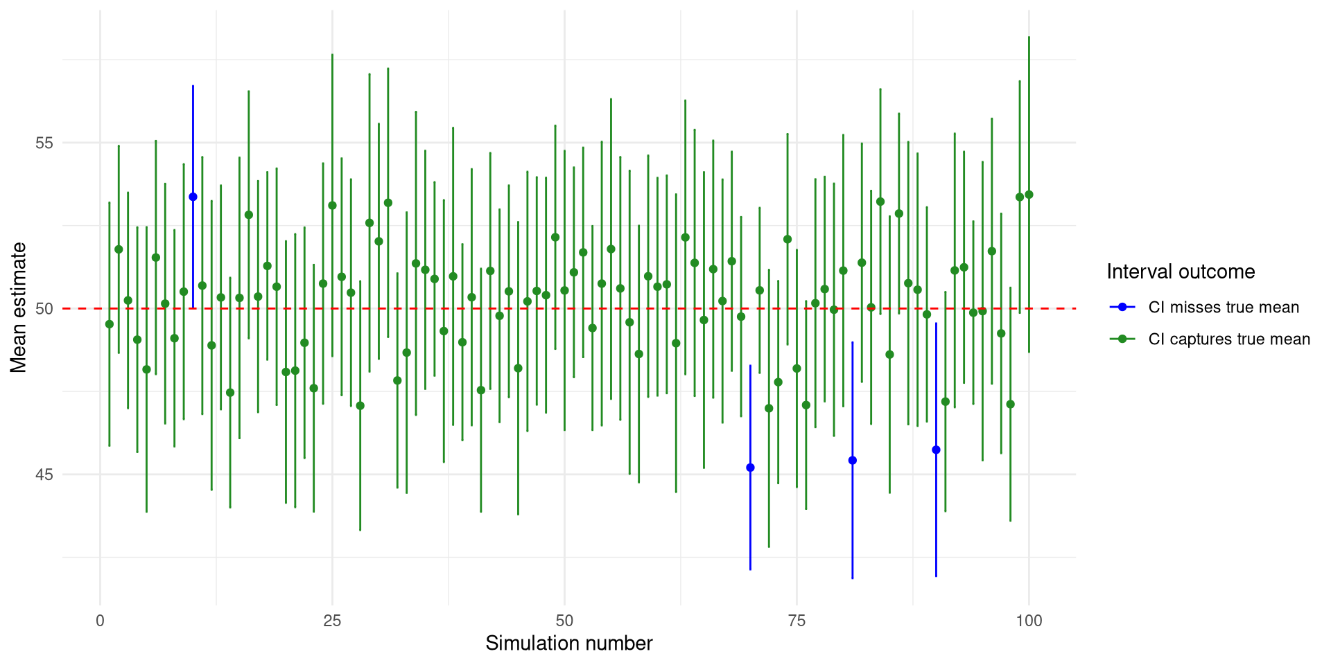
“We are 95% confident that the true mean lies between A and B.”

• This does not mean there’s a 95% chance the mean is in that interval.
• It means: if we repeated the sampling process many times, 95% of the intervals would contain the true value.

This is one of the most common misconceptions. Clarify that the confidence is in the method, not any one interval.

CI Plot

Factors Affecting CI Width

• Sample size (\(n\)): larger \(n\) → narrower CI
  
• Standard deviation (\(s\) or \(\sigma\)): more variability → wider CI
  
• Confidence level: higher confidence → wider CI

Use this to summarize what controls how “precise” our confidence interval is. Give examples of each.

Decision Making: Confidence Interval Approach

The confidence interval approach can evaluate a hypothesis test where the alternative hypothesis is \(\beta\ne\beta^*\). The confidence interval approach will result in a lower and upper bound denoted as: \((LB, UB)\).

If \(\beta^*\) is in \((LB, UB)\), then you fail to reject \(H_0\). If \(\beta^*\) is not in \((LB,UB)\), then you reject \(H_0\).

Power Analysis

1. Statistical Inference
2. Hypothesis Testing
3. Decision Making
4. Model Inference
5. Confidence Intervals
6. Power Analysis
7. Model Conditions

What is Statistical Power

• Statistical Power is the probability of correctly rejecting a false null hypothesis.
• In other words, it’s the chance of detecting a real effect when it exists.

Why Power Matters

• Low power → high risk of Type II Error (false negatives)
• High power → better chance of finding true effects
• Common threshold: 80% power

Errors in Inference

Type I	Reject \(H_0\) when true	False positive
Type II	Don’t reject \(H_0\) when false	False negative
Power	\(1 - P(\text{Type II})\)	Detecting a true effect

Power is often overlooked. It’s about how sensitive the test is to real effects. Larger samples increase power.

Type I Error (False Positive)

• Rejecting \(H_0\) when it is actually true
• Probability = \(\alpha\) (significance level)

Type I errors happen when we detect an effect that doesn’t really exist. This is controlled by our chosen alpha level.

Type II Error (False Negative)

• Failing to reject \(H_0\) when it is actually false
• Probability = \(\beta\)
• Power = \(1 - \beta\)

Type II errors are often due to small sample sizes or high variability. Power analysis helps us plan to avoid these.

Balancing Errors

• Lowering \(\alpha\) reduces Type I errors, but increases risk of Type II errors.
• To reduce both:
  • Increase sample size
  • Use more appropriate statistical tests

There’s a trade-off between these errors. We can’t eliminate both, but we can manage the risk based on the consequences of each type.

What Affects Power?

1. Effect Size
   • Bigger effects are easier to detect
2. Sample Size (\(n\))
   • Larger samples reduce standard error
3. Significance Level (\(\alpha\))
   • Higher \(\alpha\) increases power (but riskier!)
4. Variability
   • Less noise in data = better power

Boosting Power

• Power = Probability of rejecting \(H_0\) when it’s false
• Helps avoid Type II Errors
• Driven by:
  • Sample size
  • Effect size
  • \(\alpha\)
  • Variability
• Aim for 80% or higher

Model Conditions

1. Statistical Inference
2. Hypothesis Testing
3. Decision Making
4. Model Inference
5. Confidence Intervals
6. Power Analysis
7. Model Conditions

Model Conditions

When we are conducting inference with regression models, we will have to check the following conditions:

• Linearity
• Independence
• Probability Assumption
• Equal Variances
• Multicollinearity (for Multi-Regression)

Linearity

There must be a linear relationship between both the outcome variable (y) and a set of predictors (\(x_1\), \(x_2\), …).

Independence

The data points must not influence each other.

Probability Assumption

The model errors (also known as residuals) must follow a specified distribution.

• Linear Regression: Normal Distribution

• Logistic Regression: Binomial Distribution

Equal Variances

The variability of the data points must be the same for all predictor values.

Residuals

Residuals are the errors between the observed value and the estimated model. Common residuals include

• Raw Residual

• Standardized Residuals

• Jackknife (studentized) Residuals

• Deviance Residuals

• Quantized Residuals

Influential Measurements

Influential measures are statistics that determine how much a data point affects the model. Common influential measures are

• Leverages

• Cook’s Distance

Raw Residuals

\[ \hat r_i = y_i - \hat y_i \]

Residual Analysis

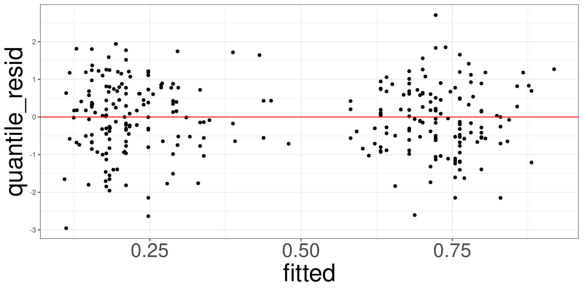
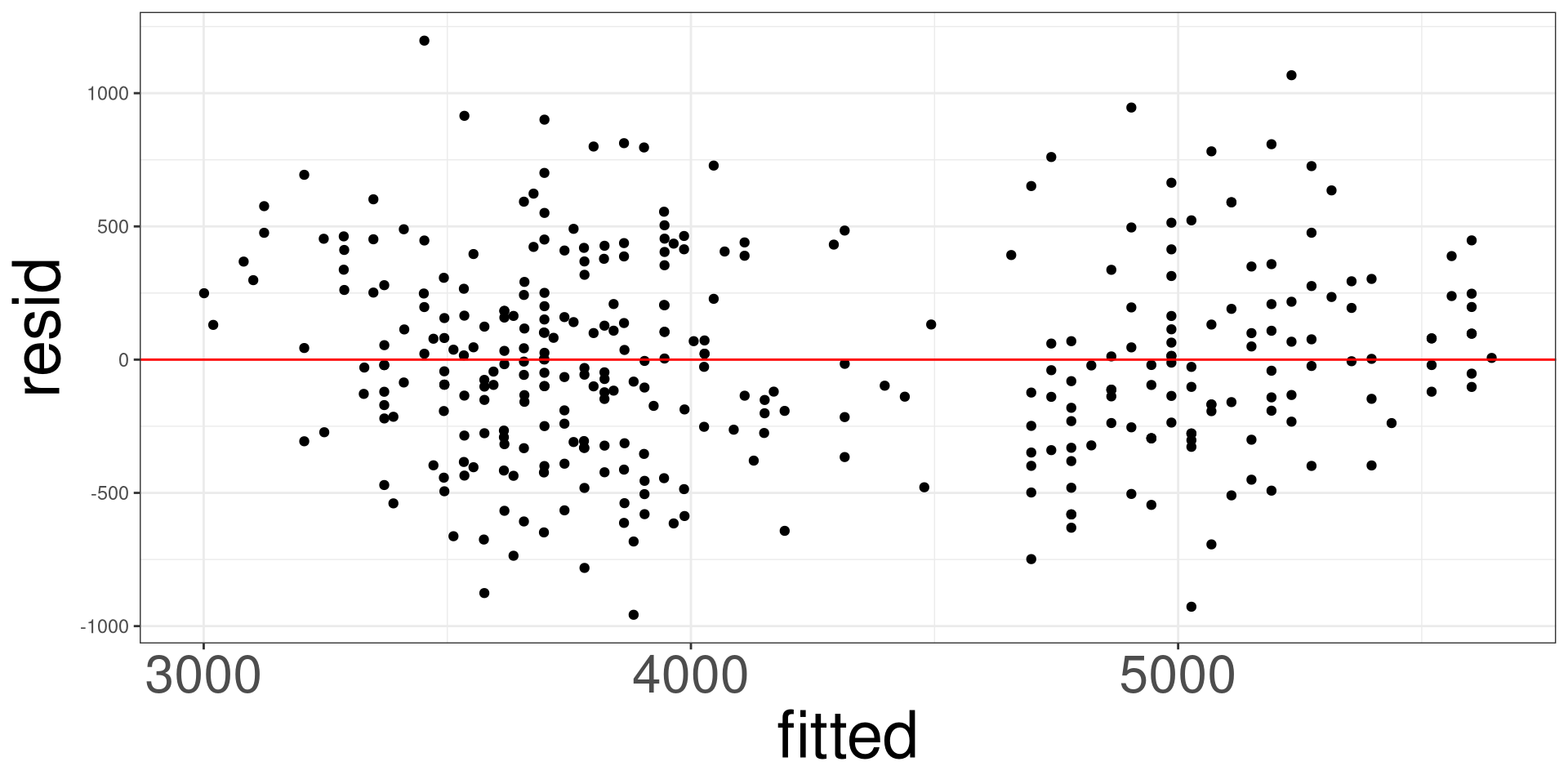
A residual analysis is used to test the assumptions of linear regression.

QQ Plot

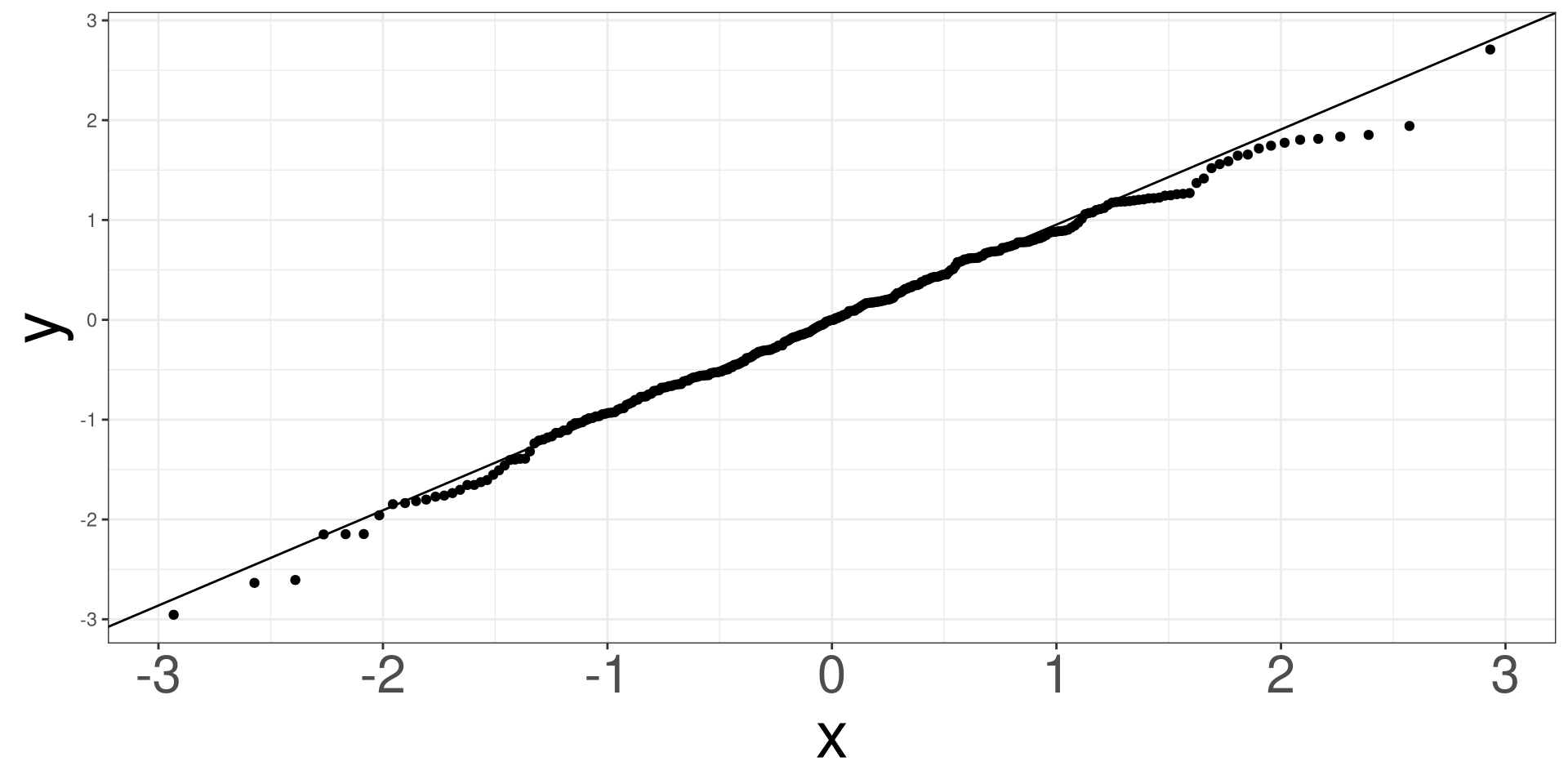
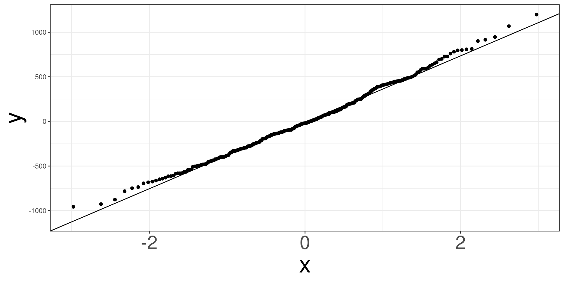
A qq (quantile-quantile) plot will plot the estimated quantiles of the residuals against the theoretical quantiles from a normal distribution function. If the points from the qq-plot lie on the \(y=x\) line, it is said that the residuals follow a normal distribution.

Residual vs Fitted Plot

This plot allows you to assess the linearity, constant variance, and identify potential outliers. Create a scatter plot between the fitted values (x-axis)

Penguins: Example

Heart: Example